On Saddle Points: a painless tutorial
Are we really stuck in the local minima rather than anything else?
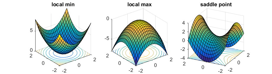
Different types of critical points
To minimize the function \(f:\mathbb{R}^n\to \mathbb{R}\), the most popular approach is to follow the opposite direction of the gradient \(\nabla f(x)\) (for simplicity, all functions we talk about are infinitely differentiable), that is,
Here \(\eta\) is a small step size. This is the gradient descent algorithm.
Whenever the gradient \(\nabla f(x)\) is nonzero, as long as we choose a small enough \(\eta\), the algorithm is guaranteed to make local progress. When the gradient \(\nabla f(x)\) is equal to \(\vec{0}\), the point is called a critical point, and gradient descent algorithm will get stuck. For (strongly) convex functions, there is a unique critical point that is also the global minimum.
However, this is not always this case. All critical points of \( f(x) \) can be further characterized by the curvature of the function in its vicinity, especially described by it’s eigenvalues of the Hessian matrix. Here I describe three possibilities as the figure above shown:
- If all eigenvalues are non-zero and positive, then the critical point is a local minimum.
- If all eigenvalues are non-zero and negative, then the critical point is a local maximum.
- If the eigenvalues are non-zero, and both positive and negative eigenvalues exist, then the critical point is a saddle point.
The proof of the above three possibilities can be shown from the reparametrization of the space of Hessian matrix. The Taylor expansion is given by(first order derivative vanishes):
And assume \(\mathbf{e_1}, \mathbf{e_2}, …, \mathbf{e_n}\) are the eigenvectors and \(\lambda_1, \lambda_2, …, \lambda_n\) are the eigenvalues correspondingly. We can make the reparametrization of the space by:
Then combined with Taylor expansion, we can get the following equation:
For the proof of the above equation, you may need to look at Spectrum Theorem, which is related to the eigenvalues and eigenvectors of symmetric matrices.
From this equation, all the three scenarios for critical points are self-explained.
First order method to escape from saddle point
A post by Rong Ge introduced a first order method to escape from saddle point. He claimed that saddle points are very unstable: if we put a ball on a saddle point, then slightly perturb it, the ball is likely to fall to a local minimum, especially when the second order term \(\frac{1}{2} (\Delta x)^T \mathbf{H} \Delta x\) is significantly smaller than 0(there is a steep direction where the function value decrease, and assume we are looking for local minimum), which is called a Strict Saddle Function in Rong Ge’s post. In this case we can use noisy gradient descent:
\(y = x - \eta \nabla f(x) + \epsilon.\)
where \(\epsilon\) is a noise vector that has mean \(\mathbf{0}\). Actually, it is the basic idea of stochastic gradient descent, which uses the gradient of a mini batch rather than the true gradient. However, the drawback of the stochastic gradient descent is not the direction, but the size of the step along each eigenvector. The step, along any direction \(\mathbf{e_i}\), is given by \(-\lambda_i \Delta \mathbf{v_i}\), when the steps taken in the direction with small absolute value of eigenvalues, the step is small. To be more concrete, an example that the curvature of the error surface may not be the same in all directions. If there is a long and narrow valley in the error surface, the component of the gradient in the direction that points along base of the valley is very small while the component perpendicular to the valley walls is quite large even though we have to move a long distance along the base and a small distance perpendicular to the walls. This phenomenon can be seen as the following figure:
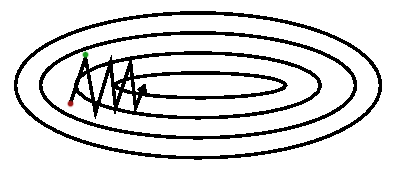
We normally move by making a step that is some constant times the negative gradient rather than a step of constant length in the direction of the negative gradient. This means that in steep regions (where we have to be careful not to make our steps too large), we move quickly, and in shallow regions (where we need to move in big steps), we move slowly.
Newton methods
To look at the detail of newton methods, you can follow the proof shown in (Sam Roweis’s) in the reference list. The newton method solves the slowness problem by rescaling the gradients in each direction with the inverse of the corresponding eigenvalue, yielding the step \(-\Delta \mathbf{v_i}\)(because \(\frac{1}{\lambda_i}\mathbf{e_i} = \mathbf{H}^{-1}\mathbf{e_i} \) ). However, this approach can result in moving in the wrong direction when the eigenvalue is negative. The newton step moves along the eigenvector in a direction opposite to the gradient descent step, thus increase the error.
From the idea of Levenberg gradient descent method, we can use damping, in which case we remove negative curvature by adding a constant \(\alpha\) to its diagonal. Informally, \(x^{k+1} = x^{k} - (\mathbf{H}+\alpha \mathbf{I})^{-1} \mathbf{g_k}\). We can view \(\alpha\) as the tradeoff between newton methods and gradient descent. When \(\alpha\) is small, it is closer to newton method, when \(\alpha\) is large, it is closer to gradient descent. In this case, we get the step \(-\frac{\lambda_i}{\lambda_i + \alpha}\Delta \mathbf{v_i}\). Therefore, obviously, the drawback of damping newton method is that it potentially has small step size in many eigen-directions incurred by large damping factor \(\alpha\).
Saddle free newton method
(Dauphin et al., 2014) introduced a method called saddle free newton method, which is a modified version of trust region approach. It minimizes first-order Taylor expansion constraint by the distance between first-order Taylor expansion and second-order Taylor expansion. By this constraint, unlike gradient descent, it can move further in the directions of low curvature; and move less in the directions of high curvature. I recommend you to read this paper throughly.
Future post
I have talked about degenerate critical point in this post, where there are only positive and zero eigenvalues in the Hessian matrix.
Marks
The slides for the talk of this blog can be found at Link. Contact me if the link is not working.
References
- Berkeley Optimization Models: Spectral Theorem
- Dauphin, Yann N., et al. Identifying and attacking the saddle point problem in high-dimensional non-convex optimization. Advances in neural information processing systems. 2014.
- Sam Roweis’s note on Levenberg-Marquardt Optimization
- Rong Ge, Escaping from Saddle Points, Off the convex path blog, 2016
- Benjamin Recht, Saddles Again, Off the convex path blog, 2016

