This post means to give you a nutshell description of bias-variance decomposition.

basic setting

We will show four key results using Bias-variance decomposition.

Let us assume $f_{true}(x_n)$ is the true model, and the observations are given by:

\[y_n = f_{true}(x_n) + \epsilon_n \qquad (1)\]

where $\epsilon_n$ are i.i.d. with zero mean and variance $\sigma^2$. Note that $f_{true}$ can be nonlinear and $\epsilon_n$ does not have to be Gaussian.

We denote the least-square estimation by

\[f_{lse}(x_{\ast}) = \tilde{x}_{\ast}^T w_{lse} \]

Where the tilde symbol means there is a constant 1 feature added to the raw data. For this derivation, we will assume that $x_{\ast}$ is fixed, although it is straightforward to generalize this.

Expected Test Error

Bias-variance comes directly out of the test error:

$$\begin{align*} \overline{teErr} &= \mathbb{E}[(observation - prediction)^2] \qquad (2.1) \\ & =\mathbb{E}_{D_{tr},D_{te}} [(y_\ast − f_{lse})^2] \qquad (2.2)\\ &= \mathbb{E}_{y_\ast,w_{lse}} [(y_\ast −f_{lse} )^2] \qquad (2.3)\\ &= \mathbb{E}_{y_\ast, w_{lse}} [(y_\ast −f_{true} + f_{true} −f_{lse})^2] \qquad (2.4) \\ &= \mathbb{E}_{y_\ast}[(y_{\ast}−f_{true})^2] + \mathbb{E}_{w_{lse}} [(f_{lse} − f_{true})^2] \qquad (2.5)\\ &= \sigma^2 + \mathbb{E} w_{lse} [(f_{lse} − \mathbb{E} w_{lse} [f_{lse}] −f_{true} + \mathbb{E}w_{lse} [f_{lse}])^2] \qquad (2.6)\\ &= \sigma^2 + \mathbb{E} w_{lse} [(f_{lse} − \mathbb{E} w_{lse} [f_{lse}])^2] + [f_{true} + \mathbb{E}w_{lse} (f_{lse})]^2 \qquad (2.7)\\ \end{align*}$$

Where equation (2.2) is the expectation over training data and testing data; and the second term in equation (2.7) is called predict variance, and the third term of it is called the square of predict bias. Thus comes the name bias-variance decomposition.

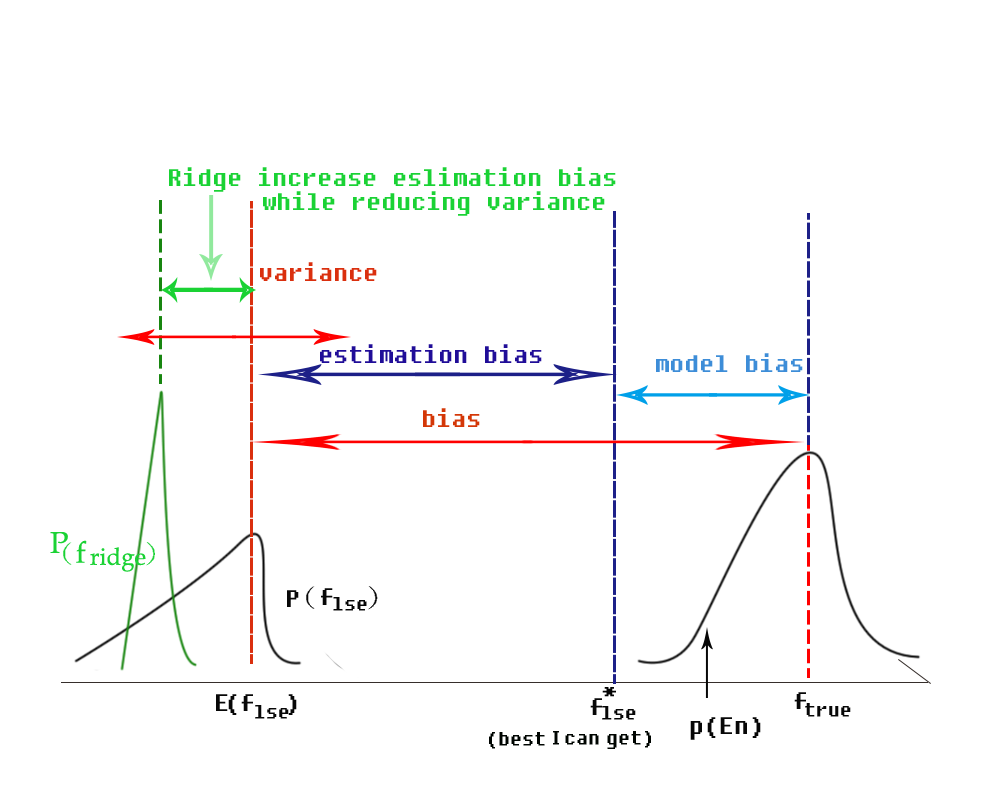
Where does the bias come from? model bias and estimation bias

As illustrated in the following figure, bias comes from model bias and estimation bias. Model bias comes from the model itself; and estimation bias comes from dataset (mainly). And bear in mind that ridge regression increases estimation bias while reducing variance(you may need to find other papers to get this idea)

References

• Kevin, Murphy. “Machine Learning: a probabilistic perspective.” (2012).
• Bishop, Christopher M. “Pattern recognition.” Machine Learning 128 (2006).
• Emtiyaz Khan’s lecture notes on PCML, 2015