This post will introduce some normalization related tricks in neural networks.

Normalization and Equalization

In image process area, the term “normalization” has many other names such as contrast stretching, histogram stretching or dynamic range expansion etc. If you have an 8-bit grayscale image, the minimum and maximum pixel values are 50 and 180, we can normalize this image to a larger dynamic range say 0 to 255. After normalize, the previous 50 becomes 0, and 180 becomes 255, the values in the middle will be scaled according to the following formula:

(I_n: new_intensity) = ((I_o: old_intensity)- (I_o_min: old_minimum_intensity)) x ((I_n_max: new_maximum_intensity) - (I_n_min: new_minimum_intensity)) / ((I_o_max: old_maximum_intensity) - (I_o_min: old_minimum_intensity)) + (I_n_min: new_minimum_intensity)

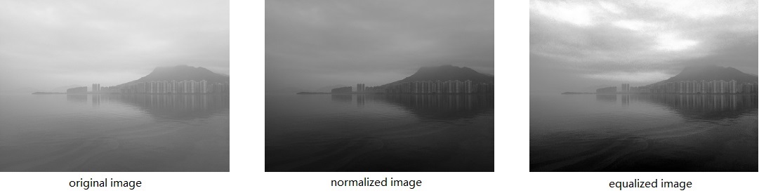
It’s a typical linear transform. Still the previous image, the pixel value 70 will become (70-50)x(255-0)/(180-50) - 0 = 39, the pixel value 130 will become (130-50)x(255-0)/(180-50) - 0 = 156. The image above shows the effect of an image before and after normalization, the third image is effect of another transform called histogram equalization, for your information, histogram equalization is different from normalization, normalization will not change your image’s histogram but equalization will. Histogram equalization doesn’t care about intensity value of the pixel, however, the ranking of the current intensity in the whole image matters a lot. The maximum intensity of the original image is 238 and the minimum is 70, implemented through OpenCV. (OpenCV’s normalization function isn’t the normalization we are talking about, if you want to repeat the effect, you have to do it yourself.) For normalization, the new intensity derives from the new and old maximum, minimum intensity; for equalization, the new intensity derives from the intensity value’s ranking in the whole image (for example, a image has 64 pixels, the intensity of a certain pixel is 90, and there are 22 pixels has a low intensity and 41 pixels has a higher intensity, the new intensity after equalization of that point is (22/64) x (255-0) = 87).

Simplified Whitening

Real whitening process is a series of linear transform to make the data have zero means and unit variances, and decorrelated. And there’s quite a lot of math, I don’t really want to talk too much about the math. (Editing formulas are quite annoying, you know.) As issued above, the propose of whitening or ICA (Independent Compoment Analysis) or sphering is to get ride of the correlations among the raw data. Let’s say, for an image, there’s a high chance that the adjacent pixel’s intensity is similar, this kind of similarity over the spatial domain is the so called correlation, and ICA is a way to reduce this similarity. Usually, in neural networks we use simplified whitening instead of original ICA, because the computation burden for ICA is just too heavy for big data (say millions of images). Too tired to explain this formula, maybe later, forgive me…

Let’s presume you have 100 grayscale images to process, each image has a width of 64 and height of 64, conventions are described as follows:

• First, calculate the mean and standard deviation (square root of variance) for pixels that has the same x and y coordinate.
• Then, for each pixel, subtract the mean and divide the standard deviation.

For example, among the 100 image, get the intensity for pixels at the position (0, 0), you will have 100 intensity values, calculate the mean and standard deviation for these 100 values. And then, for each pixel of these 100 values, subtracts the mean and divides the variance. And then repeat the same process for other pixels at other positions, in this example, you should iterate it for 64x64 times in total. After the above process, each dimension of the data set along the batch axis has a zero mean and unit variance. The similarity has already been reduced (for my understanding, the first order similarity has already gone, but the higher order similarity is still there, that’s where the real ICA takes place, to wipe out the higher order similarity). By doing whitening, the network will converge faster than without whitening.

Local Constrast Normalization (LCN)

Related papers are listed below: Why is Real-World Visual Object Recognition Hard?, published in Jan. 2008. At this time, the name is “Local input divisive normalization”. Nonlinear Image Representation Using Divisive Normalization, published in Jun. 2008. The name is “Divisive Normalization”. What is the Best Multi-Stage Architecture for Object Recognition?, released in 2009. The name is “Local Constrast Normalization”. Whitening is a way to normalize the data in different dimensions to reduce the correlations among the data, however, local contrast normalization, whose idea is inspired by computational neuroscience, aims at to make the features in feature maps more significant.

This (Local Constrast Normalization) module performs local subtraction and division normalizations, enforcing a sort of local competition between adjacent features in a feature map, and between features at the same spatial location in different feature maps.

Local contrast normalization is implemented as follows:

• First, for each pixel in a feature map, find its adjacent pixels. Let’s say the radius is 1, so there are 8 pixels around the target pixel (do the zero padding if the target is at the edge of the feature map).
• Then, compute the mean of these 9 pixels (8 neighbor pixels and the target pixel itself), subtract the mean for each one of the 9 pixels.
• Next, compute the standard deviation of these 9 pixels. And judge whether the standard deviation is larger then 1. If larger than 1, divide the target pixel’s value (after mean subtraction) by the standard deviation. If not larger, keep the target’s value as they what they are (after mean subtraction).
• At last, save the target pixel value to the same spatial position of a blank feature map as the input of the following CNN stages.

I typed the following python code to illustrate the math of the LCN:

>>> import numpy as np
>>> x = np.matrix(np.random.randint(0,255, size=(3, 3))) # generate a random 3x3 matrix, the pixel value is ranging from 0 to 255.
>>> x
matrix([[201, 239, 77], [139, 157, 23], [235, 207, 173]])
>>> mean = np.mean(x)
>>> mean
161.2222222222223
>>> x = x - mean
>>> x
matrix([[39.77777778, 77.77777778, -84.22222222], [-22.22222222, -4.22222222, -138.22222222], [73.77777778, 45.77777778, 11.77777778]])
>>> std_var = np.sqrt(np.var(x)）
>>> std_var
68.328906...
>>> std_var > 1
True
>>> LCN_value = x[(1, 1)]/std_var
>>> LCN_value
-0.0617926207...

Please be noted that the real process in the neural network is not looks like this, because the data is usually whitened before feed to the network, the image usually isn’t randomly generated and the negative value is usually set to zero in ReLU. Here, we presume that each adjacent pixel has the same importance to the contrast normalization so we calculate the mean of the 9 pixels, actually, the weights for each pixel can be various. We, presume the adjacent pixel radius is 1 and the image has only one channel, but the radius can be larger or smaller, you can pick up 4 adjacent pixels (up, down, left, right) or 24 pixels (radius is 2) or arbitrary pixels at arbitrary positions (the result may looks odd). In the third paper, they introduced the divisive normalization into neural networks, and there is variation, that is the contrast normalization among adjacent feature maps at the same spatial position (say a pixel select two adjacent feature maps, the neighbor pixel number is 3x3x3 - 1). In conv. neural network, the output of a layer may have may feature maps, and the LCN can enhance feature presentations in some feature maps at the mean time restrain the presentations in other feature maps.

Local Response Normalization (LRN)

This concept was raised in AlexNet, click here to learn more. Local response normalization algorithm was inspired by the real neurons, as the author said, “bears some resemblance to the local contrast normalization”. The common point is that they both want to introduce competitions to the neuron outputs, the difference is LRN do not subtract mean and the competition happens among the outputs of adjacent kernels at the same layer. The formula for LRN is as follows:

a(i, x, y) represents the i th conv. kernel’s output (after ReLU) at the position of (x, y) in the feature map. b(i, x, y) represents the output of local response normalization, and of course it’s also the input for the next layer. N is the number of the conv. kernel number. n is the adjacent conv. kernel number, this number is up to you. In the article they choose n = 5. k, α， β are hyper-parameters, in the article, they choose k = 2, α = 10e-4, β = 0.75. 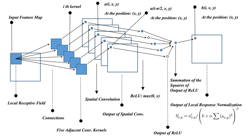Flowchart of Local Response Normalization

I drew the above figure to illustrate the process of LRN in neural network. Just a few tips here:

• This graph presumes that the i th kernel is not at the edge of the kernel space. If i equals zero or one or last or one to the last, one or two additional zero padding conv. kernels are required.
• In the article, n is 5, we presume n/2 is integer division, 5/2 = 2.
• Summation of the squares of output of ReLU stands for: for each output of ReLU, compute its square, then, add the 5 squared value together. This process is the summation term of the formula.
• I presume the necessary padding is used by the input feature map so that the output feature maps have the same size of the input feature map, if you really care. But this padding may not be quite necessary.

After knowing what LRN is, another question is: what the output of LRN looks like? Because the LRN happens after ReLU, so the inputs should all be no less than 0. The following graph tries to give you an intuitive understanding on the output of LRN, however, you still need to use your imagination.

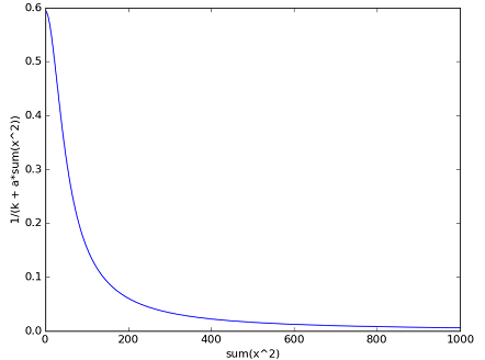
Be noted that the x axis represents the summation of the squared output of ReLU, ranging from 0 to 1000, and the y axis represents b(i, x, y) divides a(i, x, y). The hyper-parameters are set default to the article. So, the real b(i, x, y)’s value should be the the y axis’s value multiplied with the a(i, x, y), use your imagination here, two different inputs a(i, x, y) pass through this function. Since the slope at the beginning is very steep, little difference among the inputs will be significantly enlarged, this is where the competition happens. The figure was generated by the following python code:

>>> import numpy as np
>>> import matplotlib.pyplot as plt
>>> def lrn(x):
>>>...   y = 1 / (2 + (10e-4) * x ** 2) ** 0.75
>>>...   return y
>>> input = np.arange(0, 1000, 0.2)
>>> output = lrn(input)
>>> plt.plot(input, output)
>>> plt.xlabel('sum(x^2)')
>>> plt.ylabel('1 / (k + a * sum(x^2))')
>>> plt.show()

Batch Normalization

I summarized related paper in another blog. Batch normalization, at first glance, is quite difficult to understand. It truly introduced something new to CNNs, that is a kind of learnable whitening process to the inputs of the non-linear activations(ReLUs or Sigmoids). You can view the BN operation (represented as op. at the rest of this post) as a simplified whitening on the data in the intermittent layer of the neural network. In the original paper, I think the BN op. happens after the conv. op. but before the ReLU or Sigmoid op. But, BN is not that easy, because, first, the hyper-parameters “means” and “variances” are learned through back-propagation, and the training is mini-batch training either online training nor batch training. I’m going to explain these ideas below. 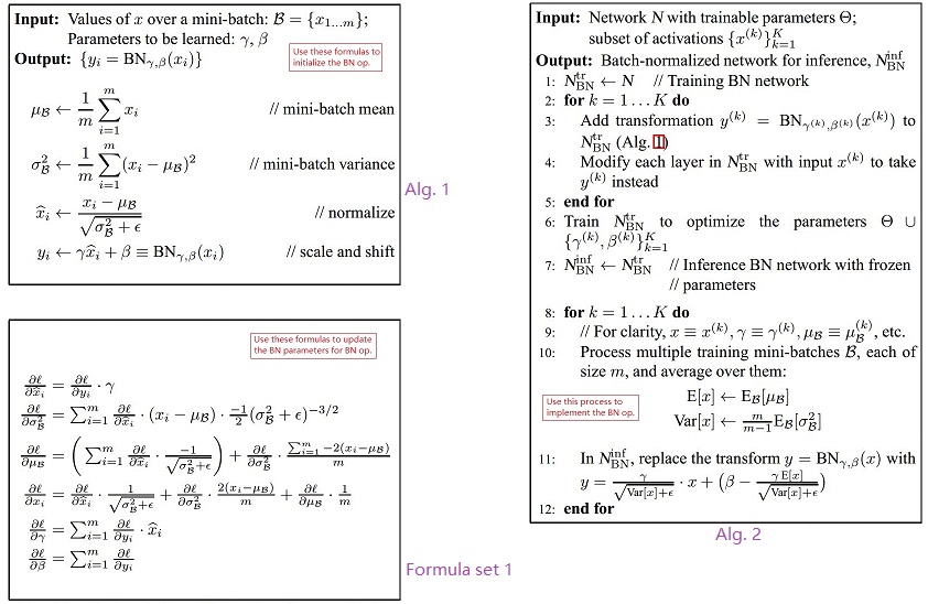First, let’s review the simplified whitening formula:

Then, follow the similar idea, batch normalization defined two trainable parameters one comes from the mean, the other comes from the variance (or variance’s square root-standard deviation), view the algorithms and formula sets in page 3 and 4 in original paper.

Online training means that when you train your network, each time you feed only one instance to your network, calculate the loss at the last layer and based on the loss of this single instance, using back-propagation to adjust your network’s parameters. Batch training means when you train your network, you feed all your data to the network, and calculate the loss of the whole dataset, based on the total loss do be BP learning. Mini-batch training means you feed a small part of your training data to the network, then, calculate the total loss of the small part of the data at the last layer, then based on the loss of this small part of data do the BP learning. Online training usually suffers from the noise the adjustment is usually quite noisy but if your training is implemented on a single thread CPU, online training is believed to be the fastest scheme and you can use larger learning rate. Batch training has a better estimation on the gradient, so the training can be less noisy, but batch training should be carefully initialized and the learning rate should be small, so the training speed is believed to be slow. Mini-batch training is a compromise between online training and the batch training. It uses a batch of data to estimate the gradient, so the learning is less noisy. Batch training and mini-batch training all can take advantage of the parallel computing such as multi-thread computing or GPU computing. So, the speed is much faster than single thread training. Batch normalization of course uses batch training. In ImageNet classification, they choose the batch size of 32, that is every time they feed 32 images to the network to calculate the loss and estimate the error. Each image is 224*224 pixels, so each batch has 50176 dimensions. Let’s take out a intermittent conv. layer to illustrate the BN op.

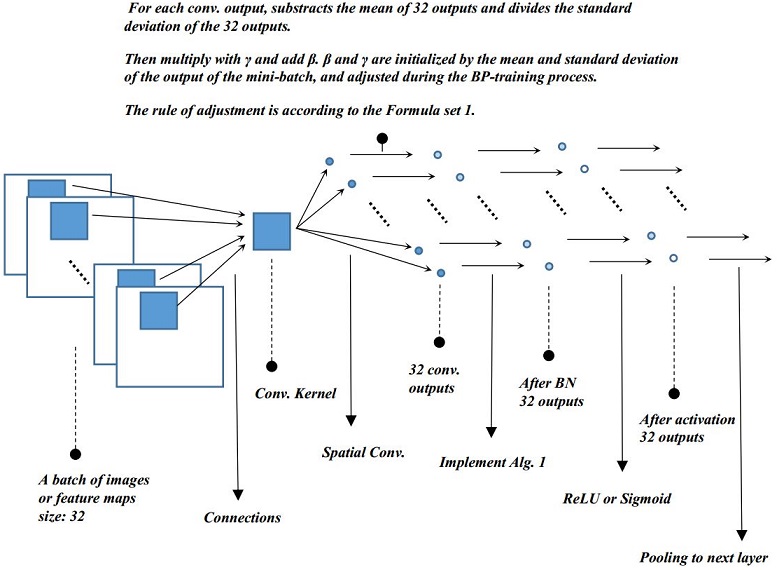
The trick part is γ and β are initialized by the batch standard deviations and means but trained subject to the loss of the network through back-propagation. Why? Why we need to train γ and β instead of using the standard deviation and mean of the batch directly, you may think it’s possibly a better way to reduce the correlations or shifts. The reason is that it can be proved or observed that by naive subtracting mean and dividing the variance, there’s no help to the network, take mean as an example, the bias unit in the network will make up the loss of the mean. In my opinion, batch normalization is trying to find a balance between the simplified whitening and raw. They issued in the paper, the initial transform is an identity transform to the data. After γ and β were trained, I believe that the transform is not identity anymore. And they also say BN is a way to solve the internal covariate shift, to solve the problem of shifting in the distribution of the inputs in different layers, according to their description, BN is a significant improvement to the network architecture, I believe it’s true but I don’t think they can really get ride of the distribution shift, as the title of the paper said, it can improve the network by “Reducing Internal Covariate Shift”. The last thing to address, when using the network trained by BN to do the inference, a further process to γ and β are needed, you can find how to implement the process according to the 8, 9, 10, 11 lines in Alg. 2. The idea is that the trained γ and β in the model need to be further normalized by the maximum likelihood estimation of global variance and mean.

License

The content of this blog itself is licensed under the Creative Commons Attribution 4.0 International License.

The containing source code (if applicable) and the source code used to format and display that content is licensed under the Apache License 2.0. Copyright [2016] [yeephycho] Licensed under the Apache License, Version 2.0 (the “License”); you may not use this file except in compliance with the License. You may obtain a copy of the License at Apache License 2.0 Unless required by applicable law or agreed to in writing, software distributed under the License is distributed on an “AS IS” BASIS, WITHOUT WARRANTIES OR CONDITIONS OF ANY KIND, either express or implied. See the License for the specific language governing permissions and limitations under the License.